[In Progress]Trading volatility term structure with ETNs and machine learning.

NOTE: This post is still work in progress and will be continually updated.

Introduction:

Volatility is often calculated using variance and standard deviation and is used to measure the amount of uncertainty or risk of an asset. To lay the groundwork for this article, there’s a few stylized fact about volatility. First, return-vol correlation: stocks and stock indices display negative correlation between variance and returns. Second, volatility clustering: variance measured for example by squared returns, displays positive correlation with its own past. Third, volatility mean-reversion: volatility tends to mean-revert towards an unconditional volatility or long-term volatility. 

VIX, often referred as the fear gauge for the market, is published by CBOE. The index is a measure of market expectations of near-term volatility conveyed by SPX options prices. 

Originally launched in 1993, it was calculated based on S&P 100 index’s 30-day at-the-money Black-Scholes implied volatility. Since 2003, it has been calculated based on S&P500 index options’ 30-day model free implied volatility. The detailed pricing model is seen below, a screenshot taken from the CBOE website.

VIX, has a wide range of application , such as forecasting variance by serving as one of the explanatory variables in the GARCH method, which I will not go into details here. 

Some mathematical review:

VIX index itself cannot be traded, however its derivatives are traded on CBOE. VIX futures and options enable various market participants to diversify their portfolio through hedging, mitigating or capitalizing on broad market volatility. Just like commodities, these players are usually hedgers, such as institutions. These pension funds, mutual funds tend to have high demand for hedges because they have a risk mandate to follow and are constrained by regulations either by the company or the government.  Then there’s speculators, such as hedge fund and me, we can speculate on the movement of the VIX, if we disagree with the market’s anticipation of future volatility, we can profit on it either through instantaneous arbitrage(HFT) or by making bullish or bearish bet on various instruments to reflect our views of future variance. Third, there’s the sellers, those are usually the market makers, options sellers. They sell volatility by pricing options. As the seller of insurance, they price the “insurance”, namely, the options implied volatility, in a way that on average, they make money. In fact, historically, average implied variance is about 21%^2, while average realized variance is about 16%^2. This implies a negative variance risk premium. If you short volatility, you make money on average, but in the case of a sharp market decline, the high left skew and fat tail of the return distribution can potentially wipe out your portfolio. Empirically, a negative return increases variance by more than a positive return of the same magnitude. Thus, this average profitability is designed to compensate for this occasional short fall. 

VIX Term Structure: 

Similar to interest rate term structure. There’s a variety of trading opportunities involved with this. If you think there’s a discrepancy between your assumption or some inefficiencies in the market due to short term local volatility spike on the futures curve, trading strategies such as butterfly, calendar spread on options futures are good ways to exploit this opportunity. Due to the VIX futures pricing nature, just like other commodities, its term structure has a contango shape with sharper decline in the front end of the curve than the backend of the curve. On top of that, the risk premia priced in by sellers as an insurance against volatility spike is contributing to its natural contango shape as well.

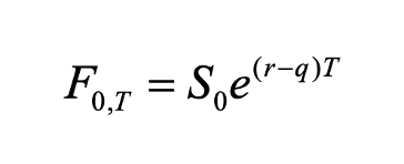
Below is the general futures pricing model with T maturity. S0 being the spot rat, r representing term rate, and q being the convenience yield less transportation cost and storage cost.

The formula below is the representation for the change in an index price that rolls over future contracts to maintain a position with fixed maturity, the RHS is essentially the weighted average of the relative change in prices of two futures contracts with different maturities plus the risk free rate, and the left hand side is the change in the index.

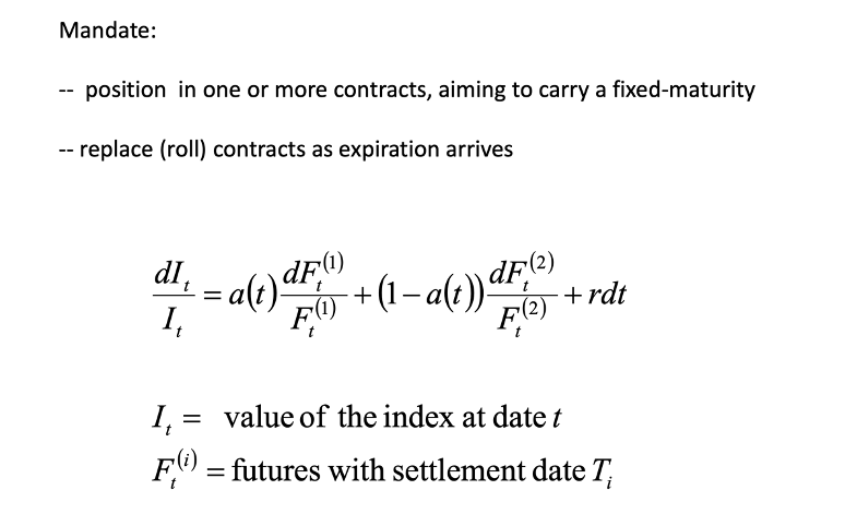
For continuous rolling, which is what VXX and VXZ represents, the weighting scheme would be the following.

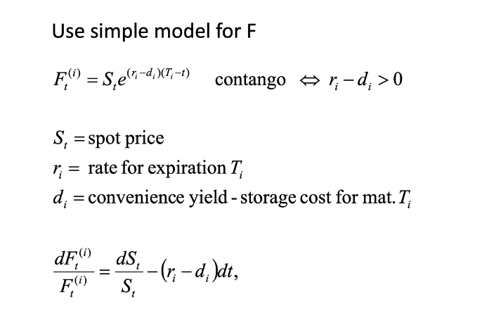
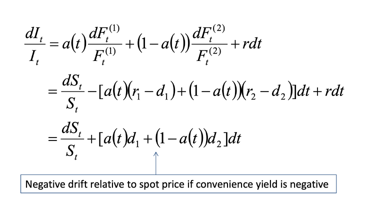
Now, we differentiate the futures price with respect to t, note that S(t) is a function itself for spot price with independent variable x. Using simple Cal1 knowledge and some simple arithmetic simplification, you’d obtain the expression of dF(t)/F(t). We’ll plug this into the Index change expression above to show that negative drift relative to spot price if convenience yield is negative. 

For VIX, the convenience yield is negative for 1. no inherent benefit of holding since volatility is not a physical asset. 2. The cost of carry due to the contango in the VIX futures market. 3. VIX is on average overpriced relative to the realized variance as an insurance premium. 4. If there’s a short-term spike in vocality, due to one of the mean-reverting characteristic of volatility, the short term d1 will be negative as market’s expecting it to drop back down to historical mean. 

Note that for cost of carry. As volatility is expressed in SPX options and OTC variance swap contract (VIX^2=1-month variance swap rate on S&P500), there’s not direct formula to calculate the cost of carry in VIX futures pricing.

The algorithm and optimization:

With all of these in mind, we can construct a strategy by shorting the front end of the curve (VXX), hedge by longing the back end of the term structure (VXZ). The weighting scheme I allocated in this specific back testing result is a vector denoted as w, where w=[xxx,xxx,xxx,xxx]

A simple but bad approximation of the contango shape of the futures curve could be dividing VIX index against VIX3M index denoted as vector IVTS (Implied volatility term structure) where IVTS=[ivtsini(1), ivtsini(2), ivtsini(3)]. This will feed into the input of the return function later. 

Now we define a function given inputs of: vector of initialized IVTSINI, vector of VXX, vector of VXZ, vector of weight, vector of cumulative return of long/short VXX,VXZ. The function will output the finalized IVTSINI values. We feed this into the optimization algorithm with set constraint based on historical distribution of IVTS value, to find the vector IVTSINI so that our return will be maximized over the back testing period from 2021.xx.xx to 2023.xx.xx.

The cumulative return function (CR) is calculated by

To choose the appropriate algorithm, we need to find out how this function behave. It’s a step wise function  

Fmincon() function is a gradient-based method that is designed to work on problems where the objective and constraint functions are both continuous and have continuous first derivatives. To find the global minima(maxima), we can use globalsearch() function in MATLAB. For this specific backtesting result, the parameters are set to….

The optimization function is a function that takes into CR-> by diving Ri into four different subspace s.t. the linear combination of WR satisfy MIN (-CR)

I’ve attached the performance and various descriptive statistics for the result below.

If you hold a market portfolio of S&P500,

Future improvement for this strategy.

1. A better curve fitting method for VIX term structure, polynomial fitting & cubic splines?
2. Using more advanced method such as maximum likelihood estimation for GARCH or other similar models. (Their performance are relatively similar)
3. More well defined risk measurement using the industry standard such as VaR and Expected Shortfall.